Document embedding using UMAP
This is a tutorial of using UMAP to embed text (but this can be extended to any collection of tokens). We are going to use the 20 newsgroups dataset which is a collection of forum posts labelled by topic. We are going to embed these documents and see that similar documents (i.e. posts in the same subforum) will end up close together. You can use this embedding for other downstream tasks, such as visualizing your corpus, or run a clustering algorithm (e.g. HDBSCAN). We will use a bag of words model and use UMAP on the count vectors as well as the TF-IDF vectors.
To start with let’s load the relevant libraries. This requires UMAP version >= 0.4.0.
import pandas as pd
import umap
import umap.plot

# Used to get the data
from sklearn.datasets import fetch_20newsgroups
from sklearn.feature_extraction.text import CountVectorizer, TfidfVectorizer

# Some plotting libraries
import matplotlib.pyplot as plt
%matplotlib notebook
from bokeh.plotting import show, save, output_notebook, output_file
from bokeh.resources import INLINE
output_notebook(resources=INLINE)
Next let’s download and explore the 20 newsgroups dataset.
%%time
dataset = fetch_20newsgroups(subset='all',
                             shuffle=True, random_state=42)
CPU times: user 280 ms, sys: 52 ms, total: 332 ms
Wall time: 460 ms
Let’s see the size of the corpus:
print(f'{len(dataset.data)} documents')
print(f'{len(dataset.target_names)} categories')
18846 documents
20 categories
Here are the categories of documents. As you can see many are related to one another (e.g. ‘comp.sys.ibm.pc.hardware’ and ‘comp.sys.mac.hardware’) but they are not all correlated (e.g. ‘sci.med’ and ‘rec.sport.baseball’).
dataset.target_names
['alt.atheism',
 'comp.graphics',
 'comp.os.ms-windows.misc',
 'comp.sys.ibm.pc.hardware',
 'comp.sys.mac.hardware',
 'comp.windows.x',
 'misc.forsale',
 'rec.autos',
 'rec.motorcycles',
 'rec.sport.baseball',
 'rec.sport.hockey',
 'sci.crypt',
 'sci.electronics',
 'sci.med',
 'sci.space',
 'soc.religion.christian',
 'talk.politics.guns',
 'talk.politics.mideast',
 'talk.politics.misc',
 'talk.religion.misc']
Let’s look at a couple of sample documents:
for idx, document in enumerate(dataset.data[:3]):
    category = dataset.target_names[dataset.target[idx]]

    print(f'Category: {category}')
    print('---------------------------')
    # Print the first 500 characters of the post
    print(document[:500])
    print('---------------------------')
Category: rec.sport.hockey
---------------------------
From: Mamatha Devineni Ratnam <mr47+@andrew.cmu.edu>
Subject: Pens fans reactions
Organization: Post Office, Carnegie Mellon, Pittsburgh, PA
Lines: 12
NNTP-Posting-Host: po4.andrew.cmu.edu


I am sure some bashers of Pens fans are pretty confused about the lack
of any kind of posts about the recent Pens massacre of the Devils. Actually,
I am  bit puzzled too and a bit relieved. However, I am going to put an end
to non-PIttsburghers' relief with a bit of praise for the Pens. Man, they
are killin
---------------------------
Category: comp.sys.ibm.pc.hardware
---------------------------
From: mblawson@midway.ecn.uoknor.edu (Matthew B Lawson)
Subject: Which high-performance VLB video card?
Summary: Seek recommendations for VLB video card
Nntp-Posting-Host: midway.ecn.uoknor.edu
Organization: Engineering Computer Network, University of Oklahoma, Norman, OK, USA
Keywords: orchid, stealth, vlb
Lines: 21

  My brother is in the market for a high-performance video card that supports
VESA local bus with 1-2MB RAM.  Does anyone have suggestions/ideas on:

  - Diamond Stealth Pro Local
---------------------------
Category: talk.politics.mideast
---------------------------
From: hilmi-er@dsv.su.se (Hilmi Eren)
Subject: Re: ARMENIA SAYS IT COULD SHOOT DOWN TURKISH PLANES (Henrik)
Lines: 95
Nntp-Posting-Host: viktoria.dsv.su.se
Reply-To: hilmi-er@dsv.su.se (Hilmi Eren)
Organization: Dept. of Computer and Systems Sciences, Stockholm University


|>The student of "regional killings" alias Davidian (not the Davidian religios sect) writes:


|>Greater Armenia would stretch from Karabakh, to the Black Sea, to the
|>Mediterranean, so if you use the term "Greater Armenia
---------------------------
Now we will create a dataframe with the target labels to be used in plotting. This will allow us to see the newsgroup when we hover over the plotted points (if using interactive plotting). This will help us evaluate (by eye) how good the embedding looks.
category_labels = [dataset.target_names[x] for x in dataset.target]
hover_df = pd.DataFrame(category_labels, columns=['category'])
Using raw counts
Next, we are going to use a bag-of-words approach (i.e. word order doesn’t matter) and construct a word document matrix. In this matrix the rows will correspond to a document (i.e. post) and each column will correspond to a particular word. The values will be the counts of how many times a given word appeared in a particular document.
We will use sklearns CountVectorizer function to do this for us along with a couple other preprocessing steps:
Split the text into tokens (i.e. words) by splitting on whitespace
Remove english stopwords (the, and, etc)
Remove all words which occur less than 5 times in the entire corpus (via the min_df parameter)
vectorizer = CountVectorizer(min_df=5, stop_words='english')
word_doc_matrix = vectorizer.fit_transform(dataset.data)
This gives us a 18846x34880 matrix where there are 18846 documents (same as above) and 34880 unique tokens. This matrix is sparse since most words do not appear in most documents.
word_doc_matrix
<18846x34880 sparse matrix of type '<class 'numpy.int64'>'
    with 1939023 stored elements in Compressed Sparse Row format>
Now we are going to do dimension reduction using UMAP to reduce the matrix from 34880 dimensions to 2 dimensions (since n_components=2). We need a distance metric and will use Hellinger distance which measures the similarity between two probability distributions. Each document has a set of counts generated by a multinomial distribution where we can use Hellinger distance to measure the similarity of these distributions.
%%time
embedding = umap.UMAP(n_components=2, metric='hellinger').fit(word_doc_matrix)
CPU times: user 2min 24s, sys: 1.18 s, total: 2min 25s
Wall time: 2min 3s
Now we have an embedding of 18846x2.
embedding.embedding_.shape
(18846, 2)
Let’s plot the embedding. If you are running this in a notebook, you should use the interactive plotting method as it lets you hover over your points and see what category they belong to.
# For interactive plotting use
# f = umap.plot.interactive(embedding, labels=dataset.target, hover_data=hover_df, point_size=1)
# show(f)
f = umap.plot.points(embedding, labels=hover_df['category'])
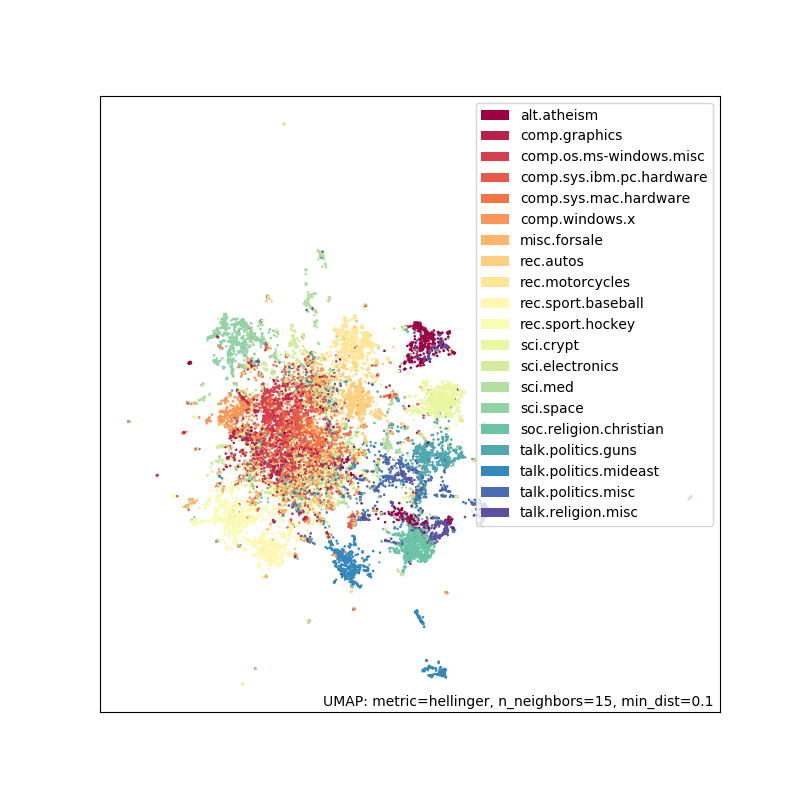
As you can see this does reasonably well. There is some separation and groups that you would expect to be similar (such as ‘rec.sport.baseball’ and ‘rec.sport.hockey’) are close together. The big clump in the middle corresponds to a lot of extremely similar newsgroups like ‘comp.sys.ibm.pc.hardware’ and ‘comp.sys.mac.hardware’.
Using TF-IDF
We will now do the same pipeline with the only change being the use of TF-IDF weighting. TF-IDF gives less weight to words that appear frequently across a large number of documents since they are more popular in general. It asserts a higher weight to words that appear frequently in a smaller subset of documents since they are probably important words for those documents.
To do the TF-IDF weighting we will use sklearns TfidfVectorizer with the same parameters as CountVectorizer above.
tfidf_vectorizer = TfidfVectorizer(min_df=5, stop_words='english')
tfidf_word_doc_matrix = tfidf_vectorizer.fit_transform(dataset.data)
We get a matrix of the same size as before:
tfidf_word_doc_matrix
<18846x34880 sparse matrix of type '<class 'numpy.float64'>'
    with 1939023 stored elements in Compressed Sparse Row format>
Again we use Hellinger distance and UMAP to embed the documents
%%time
tfidf_embedding = umap.UMAP(metric='hellinger').fit(tfidf_word_doc_matrix)
CPU times: user 2min 19s, sys: 1.27 s, total: 2min 20s
Wall time: 1min 57s
# For interactive plotting use
# fig = umap.plot.interactive(tfidf_embedding, labels=dataset.target, hover_data=hover_df, point_size=1)
# show(fig)
fig = umap.plot.points(tfidf_embedding, labels=hover_df['category'])
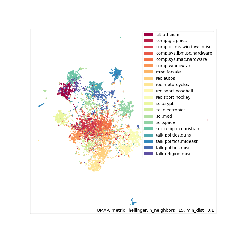
The results look fairly similar to before but this can be a useful trick to have in your toolbox.
Potential applications
Now that we have an embedding, what can we do with it?
Explore/visualize your corpus to identify topics/trends
Cluster the embedding to find groups of related documents
Look for nearest neighbours to find related documents
Look for anomalous documents