How UMAP Works
UMAP is an algorithm for dimension reduction based on manifold learning techniques and ideas from topological data analysis. It provides a very general framework for approaching manifold learning and dimension reduction, but can also provide specific concrete realizations. This article will discuss how the algorithm works in practice. There exist deeper mathematical underpinnings, but for the sake of readability by a general audience these will merely be referenced and linked. If you are looking for the mathematical description please see the UMAP paper.
To begin making sense of UMAP we will need a little bit of mathematical background from algebraic topology and topological data analysis. This will provide a basic algorithm that works well in theory, but unfortunately not so well in practice. The next step will be to make use of some basic Riemannian geometry to bring real world data a little closer to the underlying assumptions of the topological data analysis algorithm. Unfortunately this will introduce new complications, which will be resolved through a combination of deep math (details of which will be elided) and fuzzy logic. We can then put the pieces back together again, and combine them with a new approach to finding a low dimensional representation more fitting to the new data structures at hand. Putting this all together we arrive at the basic UMAP algorithm.
Topological Data Analysis and Simplicial Complexes
Simplicial complexes are a means to construct topological spaces out of simple combinatorial components. This allows one to reduce the complexities of dealing with the continuous geometry of topological spaces to the task of relatively simple combinatorics and counting. This method of taming geometry and topology will be fundamental to our approach to topological data analysis in general, and dimension reduction in particular.
The first step is to provide some simple combinatorial building blocks called *simplices*. Geometrically a simplex is a very simple way to build a \(k\)-dimensional object. A \(k\) dimensional simplex is called a \(k\)-simplex, and it is formed by taking the convex hull of \(k+1\) independent points. Thus a 0-simplex is a point, a 1-simplex is a line segment (between two zero simplices), a 2-simplex is a triangle (with three 1-simplices as “faces”), and a 3-simplex is a tetrahedron (with four 2-simplices as “faces”). Such a simple construction allows for easy generalization to arbitrary dimensions.
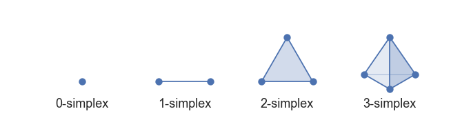
Low dimensional simplices
This has a very simple combinatorial underlying structure, and ultimately one can regard a \(k\)-simplex as an arbitrary set of \(k+1\) objects with faces (and faces of faces etc.) given by appropriately sized subsets – one can always provide a “geometric realization” of this abstract set description by constructing the corresponding geometric simplex.
Simplices can provide building blocks, but to construct interesting topological spaces we need to be able to glue together such building blocks. This can be done by constructing a *simplicial complex*. Ostensibly a simplicial complex is a set of simplices glued together along faces. More explicitly a simplicial complex \(\mathcal{K}\) is a set of simplices such that any face of any simplex in \(\mathcal{K}\) is also in \(\mathcal{K}\) (ensuring all faces exist), and the intersection of any two simplices in \(\mathcal{K}\) is a face of both simplices. A large class of topological spaces can be constructed in this way – just gluing together simplices of various dimensions along their faces. A little further abstraction will get to *simplicial sets* which are purely combinatorial, have a nice category theoretic presentation, and can generate a much broader class of topological spaces, but that will take us too far afield for this article. The intuition of simplicial complexes will be enough to illustrate the relevant ideas and motivation.
How does one apply these theoretical tools from topology to finite sets of data points? To start we’ll look at how one might construct a simplicial complex from a topological space. The tool we will consider is the construction of a Čech complex given an open cover of a topological space. That’s a lot of verbiage if you haven’t done much topology, but we can break it down fairly easily for our use case. An open cover is essentially just a family of sets whose union is the whole space, and a Čech complex is a combinatorial way to convert that into a simplicial complex. It works fairly simply: let each set in the cover be a 0-simplex; create a 1-simplex between two such sets if they have a non-empty intersection; create a 2-simplex between three such sets if the triple intersection of all three is non-empty; and so on. Now, that doesn’t sound very advanced – just looking at intersections of sets. The key is that the background topological theory actually provides guarantees about how well this simple process can produce something that represents the topological space itself in a meaningful way (the Nerve theorem is the relevant result for those interested). Obviously the quality of the cover is important, and finer covers provide more accuracy, but the reality is that despite its simplicity the process captures much of the topology.
Next we need to understand how to apply that process to a finite set of data samples. If we assume that the data samples are drawn from some underlying topological space then to learn about the topology of that space we need to generate an open cover of it. If our data actually lie in a metric space (i.e. we can measure distance between points) then one way to approximate an open cover is to simply create balls of some fixed radius about each data point. Since we only have finite samples, and not the topological space itself, we cannot be sure it is truly an open cover, but it might be as good an approximation as we could reasonably expect. This approach also has the advantage that the Čech complex associated to the cover will have a 0-simplex for each data point.
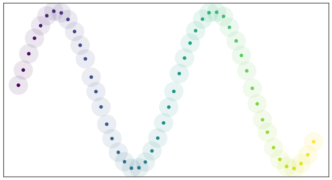
To demonstrate the process let’s consider a test dataset like this
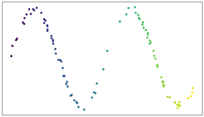
Test data set of a noisy sine wave
If we fix a radius we can then picture the open sets of our cover as circles (since we are in a nice visualizable two dimensional case). The result is something like this
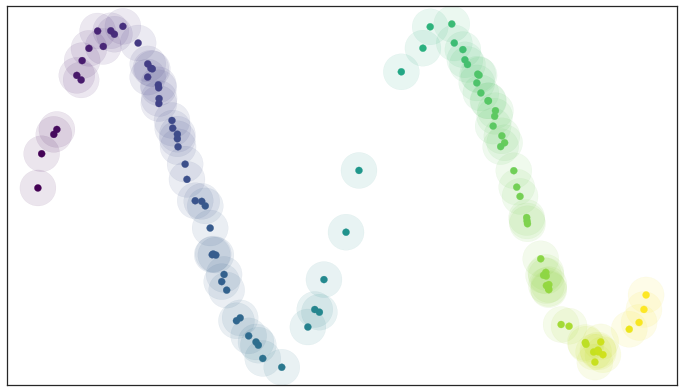
A basic open cover of the test data
We can then depict the the simplicial complex of 0-, 1-, and 2-simplices as points, lines, and triangles
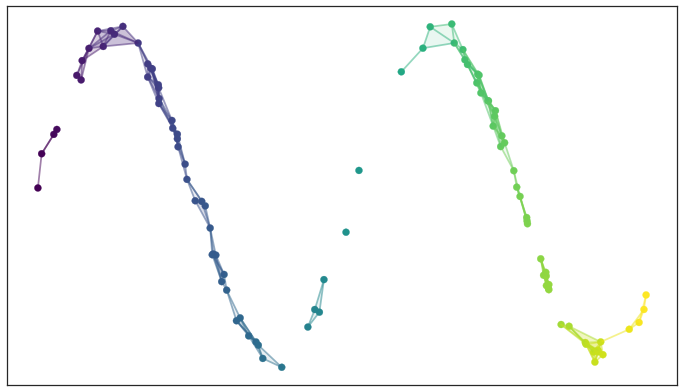
A simplicial complex built from the test data
It is harder to easily depict the higher dimensional simplices, but you can imagine how they would fit in. There are two things to note here: first, the simplicial complex does a reasonable job of starting to capture the fundamental topology of the dataset; second, most of the work is really done by the 0- and 1-simplices, which are easier to deal with computationally (it is just a graph, in the nodes and edges sense). The second observation motivates the Vietoris-Rips complex, which is similar to the Čech complex but is entirely determined by the 0- and 1-simplices. Vietoris-Rips complexes are much easier to work with computationally, especially for large datasets, and are one of the major tools of topological data analysis.
If we take this approach to get a topological representation then we can build a dimension reduction algorithm by finding a low dimensional representation of the data that has a similar topological representation. If we only care about the 0- and 1-simplices then the topological representation is just a graph, and finding a low dimensional representation can be described as a graph layout problem. If one wants to use, for example, spectral methods for graph layout then we arrive at algorithms like Laplacian eigenmaps and Diffusion maps. Force directed layouts are also an option, and provide algorithms closer to MDS or Sammon mapping in flavour.
I would not blame those who have read this far to wonder why we took such an abstract roundabout road to simply building a neighborhood-graph on the data and then laying out that graph. There are a couple of reasons. The first reason is that the topological approach, while abstract, provides sound theoretical justification for what we are doing. While building a neighborhood-graph and laying it out in lower dimensional space makes heuristic sense and is computationally tractable, it doesn’t provide the same underlying motivation of capturing the underlying topological structure of the data faithfully – for that we need to appeal to the powerful topological machinery I’ve hinted lies in the background. The second reason is that it is this more abstract topological approach that will allow us to generalize the approach and get around some of the difficulties of the sorts of algorithms described above. While ultimately we will end up with a process that is fairly simple computationally, understanding why various manipulations matter is important to truly understanding the algorithm (as opposed to merely computing with it).
Adapting to Real World Data
The approach described above provides a nice theory for why a neighborhood graph based approach should capture manifold structure when doing dimension reduction. The problem tends to come when one tries to put the theory into practice. The first obvious difficulty (and we can see it even our example above) is that choosing the right radius for the balls that make up the open cover is hard. If you choose something too small the resulting simplicial complex splits into many connected components. If you choose something too large the simplicial complex turns into just a few very high dimensional simplices (and their faces etc.) and fails to capture the manifold structure anymore. How should one solve this?
The dilemma is in part due to the theorem (called the Nerve theorem) that provides our justification that this process captures the topology. Specifically, the theorem says that the simplicial complex will be (homotopically) equivalent to the union of the cover. In our case, working with finite data, the cover, for certain radii, doesn’t cover the whole of the manifold that we imagine underlies the data – it is that lack of coverage that results in the disconnected components. Similarly, where the points are too bunched up, our cover does cover “too much” and we end up with higher dimensional simplices than we might ideally like. If the data were uniformly distributed across the manifold then selecting a suitable radius would be easy – the average distance between points would work well. Moreover with a uniform distribution we would be guaranteed that our cover would actually cover the whole manifold with no “gaps” and no unnecessarily disconnected components. Similarly, we would not suffer from those unfortunate bunching effects resulting in unnecessarily high dimensional simplices.
If we consider data that is uniformly distributed along the same manifold it is not hard to pick a good radius (a little above half the average distance between points) and the resulting open cover looks pretty good:
Open balls over uniformly_distributed_data
Because the data is evenly spread we actually cover the underlying manifold and don’t end up with clumping. In other words, all this theory works well assuming that the data is uniformly distributed over the manifold.
Unsurprisingly this uniform distribution assumption crops up elsewhere in manifold learning. The proofs that Laplacian eigenmaps work well require the assumption that the data is uniformly distributed on the manifold. Clearly if we had a uniform distribution of points on the manifold this would all work a lot better – but we don’t! Real world data simply isn’t that nicely behaved. How can we resolve this? By turning the problem on its head: assume that the data is uniformly distributed on the manifold, and ask what that tells us about the manifold itself. If the data looks like it isn’t uniformly distributed that must simply be because the notion of distance is varying across the manifold – space itself is warping: stretching or shrinking according to where the data appear sparser or denser.
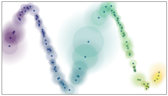
By assuming that the data is uniformly distributed we can actually compute (an approximation of) a local notion of distance for each point by making use of a little standard Riemannian geometry. In practical terms, once you push the math through, this turns out to mean that a unit ball about a point stretches to the k-th nearest neighbor of the point, where k is the sample size we are using to approximate the local sense of distance. Each point is given its own unique distance function, and we can simply select balls of radius one with respect to that local distance function!
Open balls of radius one with a locally varying metric
This theoretically derived result matches well with many traditional graph based algorithms: a standard approach for such algorithms is to use a k-neighbor graph instead of using balls of some fixed radius to define connectivity. What this means is that each point in the dataset is given an edge to each of its k nearest neighbors – the effective result of our locally varying metric with balls of radius one. Now, however, we can explain why this works in terms of simplicial complexes and the Nerve theorem.
Of course we have traded choosing the radius of the balls for choosing a value for k. However it is often easier to pick a resolution scale in terms of number of neighbors than it is to correctly choose a distance. This is because choosing a distance is very dataset dependent: one needs to look at the distribution of distances in the dataset to even begin to select a good value. In contrast, while a k value is still dataset dependent to some degree, there are reasonable default choices, such as the 10 nearest neighbors, that should work acceptably for most datasets.
At the same time the topological interpretation of all of this gives us a more meaningful interpretation of k. The choice of k determines how locally we wish to estimate the Riemannian metric. A small choice of k means we want a very local interpretation which will more accurately capture fine detail structure and variation of the Riemannian metric. Choosing a large k means our estimates will be based on larger regions, and thus, while missing some of the fine detail structure, they will be more broadly accurate across the manifold as a whole, having more data to make the estimate with.
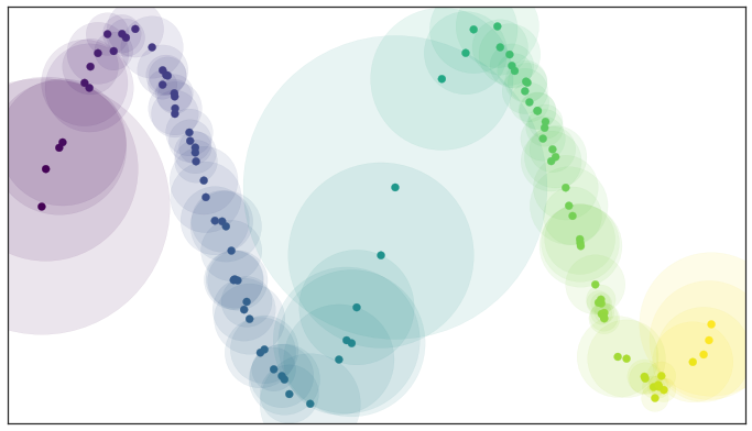
We also get a further benefit from this Riemannian metric based approach: we actually have a local metric space associated to each point, and can meaningfully measure distance, and thus we could weight the edges of the graph we might generate by how far apart (in terms of the local metric) the points on the edges are. In slightly more mathematical terms we can think of this as working in a fuzzy topology where being in an open set in a cover is no longer a binary yes or no, but instead a fuzzy value between zero and one. Obviously the certainty that points are in a ball of a given radius will decay as we move away from the center of the ball. We could visualize such a fuzzy cover as looking something like this
Fuzzy open balls of radius one with a locally varying metric
None of that is very concrete or formal – it is merely an intuitive picture of what we would like to have happen. It turns out that we can actually formalize all of this by stealing the singular set and geometric realization functors from algebraic topology and then adapting them to apply to metric spaces and fuzzy simplicial sets. The mathematics involved in this is outside the scope of this exposition, but for those interested you can look at the original work on this by David Spivak and our paper. It will have to suffice to say that there is some mathematical machinery that lets us realize this intuition in a well defined way.
This resolves a number of issues, but a new problem presents itself when we apply this sort of process to real data, especially in higher dimensions: a lot of points become essentially totally isolated. One would imagine that this shouldn’t happen if the manifold the data was sampled from isn’t pathological. So what property are we expecting that manifold to have that we are somehow missing with the current approach? What we need to add is the idea of local connectivity.
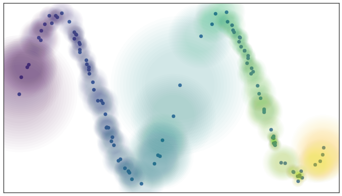
Note that this is not a requirement that the manifold as a whole be connected – it can be made up of many connected components. Instead it is a requirement that at any point on the manifold there is some sufficiently small neighborhood of the point that is connected (this “in a sufficiently small neighborhood” is what the “local” part means). For the practical problem we are working with, where we only have a finite approximation of the manifold, this means that no point should be completely isolated – it should connect to at least one other point. In terms of fuzzy open sets what this amounts to is that we should have complete confidence that the open set extends as far as the closest neighbor of each point. We can implement this by simply having the fuzzy confidence decay in terms of distance beyond the first nearest neighbor. We can visualize the result in terms of our example dataset again.
Local connectivity and fuzzy open sets
Again this can be formalized in terms of the aforementioned mathematical machinery from algebraic topology. From a practical standpoint this plays an important role for high dimensional data – in high dimensions distances tend to be larger, but also more similar to one another (see the curse of dimensionality). This means that the distance to the first nearest neighbor can be quite large, but the distance to the tenth nearest neighbor can often be only slightly larger (in relative terms). The local connectivity constraint ensures that we focus on the difference in distances among nearest neighbors rather than the absolute distance (which shows little differentiation among neighbors).
Just when we think we are almost there, having worked around some of the issues of real world data, we run aground on a new obstruction: our local metrics are not compatible! Each point has its own local metric associated to it, and from point a’s perspective the distance from point a to point b might be 1.5, but from the perspective of point b the distance from point b to point a might only be 0.6. Which point is right? How do we decide? Going back to our graph based intuition we can think of this as having directed edges with varying weights something like this.
Edges with incompatible weights
Between any two points we might have up to two edges and the weights on those edges disagree with one another. There are a number of options for what to do given two disagreeing weights – we could take the maximum, the minimum, the arithmetic mean, the geometric mean, or something else entirely. What we would really like is some principled way to make the decision. It is at this point that the mathematical machinery we built comes into play. Mathematically we actually have a family of fuzzy simplicial sets, and the obvious choice is to take their union – a well defined operation. There are a a few ways to define fuzzy unions, depending on the nature of the logic involved, but here we have relatively clear probabilistic semantics that make the choice straightforward. In graph terms what we get is the following: if we want to merge together two disagreeing edges with weight a and b then we should have a single edge with combined weight \(a + b - a \cdot b\). The way to think of this is that the weights are effectively the probabilities that an edge (1-simplex) exists. The combined weight is then the probability that at least one of the edges exists.
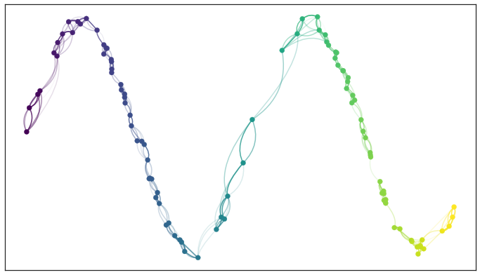
If we apply this process to union together all the fuzzy simplicial sets we end up with a single fuzzy simplicial complex, which we can again think of as a weighted graph. In computational terms we are simply applying the edge weight combination formula across the whole graph (with non-edges having a weight of 0). In the end we have something that looks like this.
Graph with combined edge weights
So in some sense in the end we have simply constructed a weighted graph (although we could make use of higher dimensional simplices if we wished, just at significant extra computational cost). What the mathematical theory lurking in the background did for us is determine why we should construct this graph. It also helped make the decisions about exactly how to compute things, and gives a concrete interpretation of what this graph means. So while in the end we just constructed a graph, the math answered the important questions to get us here, and can help us determine what to do next.
So given that we now have a fuzzy topological representation of the data (which the math says will capture the topology of the manifold underlying the data), how do we go about converting that into a low dimensional representation?
Finding a Low Dimensional Representation
Ideally we want the low dimensional representation to have as similar a fuzzy topological structure as possible. The first question is how do we determine the fuzzy topological structure of a low dimensional representation, and the second question is how do we find a good one.
The first question is largely already answered – we should presumably
follow the same procedure we just used to find the fuzzy topological
structure of our data. There is a quirk, however: this time around the
data won’t be lying on some manifold, we’ll have a low dimensional
representation that is lying on a very particular manifold. That
manifold is, of course, just the low dimensional euclidean space we are
trying to embed into. This means that all the effort we went to
previously to make vary the notion of distance across the manifold is
going to be misplaced when working with the low dimensional
representation. We explicitly want the distance on the manifold to be
standard euclidean distance with respect to the global coordinate
system, not a varying metric. That saves some trouble. The other quirk
is that we made use of the distance to the nearest neighbor, again
something we computed given the data. This is also a property we would
like to be globally true across the manifold as we optimize toward a
good low dimensional representation, so we will have to accept it as a
hyper-parameter min_dist to the algorithm.
The second question, ‘how do we find a good low dimensional representation’, hinges on our ability to measure how “close” a match we have found in terms of fuzzy topological structures. Given such a measure we can turn this into an optimization problem of finding the low dimensional representation with the closest fuzzy topological structure. Obviously if our measure of closeness turns out to have various properties the nature of the optimization techniques we can apply will differ.
Going back to when we were merging together the conflicting weights associated to simplices, we interpreted the weights as the probability of the simplex existing. Thus, since both topological structures we are comparing share the same 0-simplices, we can imagine that we are comparing the two vectors of probabilities indexed by the 1-simplices. Given that these are Bernoulli variables (ultimately the simplex either exists or it doesn’t, and the probability is the parameter of a Bernoulli distribution), the right choice here is the cross entropy.
Explicitly, if the set of all possible 1-simplices is \(E\), and we have weight functions such that \(w_h(e)\) is the weight of the 1-simplex \(e\) in the high dimensional case and \(w_l(e)\) is the weight of \(e\) in the low dimensional case, then the cross entropy will be
This might look complicated, but if we go back to thinking in terms of a graph we can view minimizing the cross entropy as a kind of force directed graph layout algorithm.
The first term, \(w_h(e) \log\left(\frac{w_h(e)}{w_l(e)}\right)\), provides an attractive force between the points \(e\) spans whenever there is a large weight associated to the high dimensional case. This is because this term will be minimized when \(w_l(e)\) is as large as possible, which will occur when the distance between the points is as small as possible.
In contrast the second term, \((1 - w_h(e)) \log\left(\frac{1 - w_h(e)}{1 - w_l(e)}\right)\), provides a repulsive force between the ends of \(e\) whenever \(w_h(e)\) is small. This is because the term will be minimized by making \(w_l(e)\) as small as possible.
On balance this process of pull and push, mediated by the weights on edges of the topological representation of the high dimensional data, will let the low dimensional representation settle into a state that relatively accurately represents the overall topology of the source data.
The UMAP Algorithm
Putting all these pieces together we can construct the UMAP algorithm. The first phase consists of constructing a fuzzy topological representation, essentially as described above. The second phase is simply optimizing the low dimensional representation to have as close a fuzzy topological representation as possible as measured by cross entropy.
When constructing the initial fuzzy topological representation we can take a few shortcuts. In practice, since fuzzy set membership strengths decay away to be vanishingly small, we only need to compute them for the nearest neighbors of each point. Ultimately that means we need a way to quickly compute (approximate) nearest neighbors efficiently, even in high dimensional spaces. We can do this by taking advantage of the Nearest-Neighbor-Descent algorithm of Dong et al. The remaining computations are now only dealing with local neighbors of each point and are thus very efficient.
In optimizing the low dimensional embedding we can again take some shortcuts. We can use stochastic gradient descent for the optimization process. To make the gradient descent problem easier it is beneficial if the final objective function is differentiable. We can arrange for that by using a smooth approximation of the actual membership strength function for the low dimensional representation, selecting from a suitably versatile family. In practice UMAP uses the family of curves of the form \(\frac{1}{1 + a x^{2b}}\). Equally we don’t want to have to deal with all possible edges, so we can use the negative sampling trick (as used by word2vec and LargeVis), to simply sample negative examples as needed. Finally since the Laplacian of the topological representation is an approximation of the Laplace-Beltrami operator of the manifold we can use spectral embedding techniques to initialize the low dimensional representation into a good state.
Putting all these pieces together we arrive at an algorithm that is fast and scalable, yet still built out of sound mathematical theory. Hopefully this introduction has helped provide some intuition for that underlying theory, and for how the UMAP algorithm works in practice.